Do you plan on flying a quad copter? Well, what if you could stream in data wirelessly?! Then you could replay your quadcopter in 3D motion and track its battery data over the course of your flight. This will mainly comprise of wirelessly connecting to the ardupilot mega (APM) quad copter through an XBee connection. One XBee will be connected to the computer and the other will be connected to the telemetry port on the quad copter. Follow the following wiki page for instructions on how to construct this: http://copter.ardupilot.com/wiki/xbee-radios/
Now that you have fully hooked up your XBees and quad copter, now we can talk about MavLink! MavLink is a software program that takes input data from the XBee and determines location, speed, GPS location, etc. for the quad copter. Follow the link for instructions on installing MavLink and follow the tutorial to learn about all the cool things it can do! http://qgroundcontrol.org/mavlink/start
When you start MavLink, your window should look like that of Figure 1.
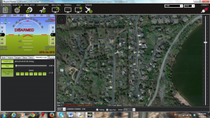
Figure 1
The next step will be to connect your quad copter to your computer. With your XBee hooked up to your telemetry port on the quad copter, you will need to connect your ground XBee to your computer using a Digi Evaluation board. Do take note of which COM port you are plugged in and select that at the top right of the MavLink window. Then click “Connect.” If all goes well, the “Connect” button should turn green.
If you are an experience quad copter flier, you will already know about the lock function. When you lock your remote controller to the quad copter, it takes note of its current position and begins logging the data and sending it via XBee. It will stop when you unlock your controller from the quad copter.
After you have taken a flight, you are now ready to access your logged data. Click on the “Load Log” button and a window like that of Figure 2 will pop up. Click “Convert to Text.” This will save the data in a text file to be used next.
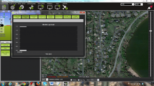
Figure 2
For the following, you will need to install TLogDataExtractor. The instructions for doing so can be found here: http://diydrones.com/profiles/blogs/extracting-data-from-tlog-files-for-plotting-in-excel
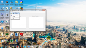
Figure 3
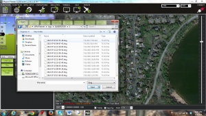
Figure 4
When you have successfully installed it, go ahead and open it. On the window, select “File” and then “Open” as shown in Figure 3. Select the text file of your data like in Figure 4.
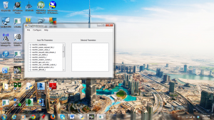
Figure 5
If all is well, your window should now look like Figure 5. We want to only select a few parameters to organize into our data. Select the following in the order given:
- mavlink_global_position_int_t.lat
- mavlink_global_position_int_t.lon
- mavlink_global_position_int_t.alt
- mavlink_sys_status_t.voltage_battery
- mavlink_sys_status_t.current_battery
- mavlink_sys_status_t.battery_remaining
- mavlink_gps_raw_int._t.vel
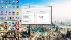
Figure 6
Your window should now look like that of Figure 6. Go ahead and save the file. The program will organize the data into a CSV file. When you open it, it should look like Figures 7 and 8 (except the last column).
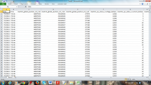
Figure 7
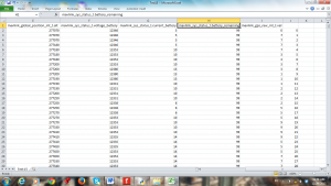
Figure 8
In the last column, starting with the first line of data, enter 0 and then increment by 1 going down the column of data.
You are now ready to write some code! You will need to download and install VPython, which can be found at http://vpython.org/. In your IDE, enter in the following code. Make sure you enter in the name of your file including .csv and ensure it is in the same folder as your program!
from visual import *
from time import clock
from visual.graph import *import csv
ifile = open(‘ENTER THE NAME OF YOUR FILE HERE’)reader = csv.reader(ifile)
#Shows path of quadcopter
L = 100e2
r = 2e2
rownum = 0
x = 0
y = 0
z = 0
scene.forward = (-1,-1,-1)
scene.width = 750
scene.height = 500
xaxis = curve(pos = [(0,0,0), (L,0,0)], color = (0.5,0.5,0.5))
yaxis = curve(pos = [(0,0,0), (0,L,0)], color = (0.5,0.5,0.5))
zaxis = curve(pos = [(0,0,0), (0,0,L)], color = (0.5,0.5,0.5))
Copter = sphere(pos = (x,y,z), radius = r, color = color.blue)
trail = curve(color = color.green)
gdisplay(width=616, height=250, x=750, y=0, title = 'Voltage vs. Time', xtitle = 'Time (sec)', ytitle = 'Voltage (Volts)', ymin = 9, ymax = 13)
VoltGraph = gcurve(color = color.red)
gdisplay(width=616, height=250, x=750, y=250, title = 'Current vs. Time', xtitle = 'Time (sec)', ytitle = 'Current (Amps)')
CurrentGraph = gcurve(color = color.yellow)
gdisplay(width=616, height=250, x=750, y=500, title = 'Battery Remaining vs. Time', xtitle = 'Time (sec)', ytitle = 'Battery Remaining (%)')
BattRemain = gcurve(color = color.cyan)
gdisplay(width=750, height=250, x=0, y=500, title = 'Speed vs. Time', xtitle = 'Time (sec)', ytitle = 'Speed (m/s)')
VelGraph = gcurve(color = color.orange)
for row in reader:
rate(50)
#skip header
if rownum == 0:
header = row
elif rownum == 1:
values = row
x0 = float(values[3])*1.1
y0 = float(values[4])*.1
z0 = float(values[2])*1.1
Copter.pos = (x,y,z)
trail.append(pos = Copter.pos)
VoltGraph.plot(pos = (float(values[9])*.2576095,float(values[5])*.001))
CurrentGraph.plot(pos = (float(values[9])*.2576095,float(values[6])*.001))
BattRemain.plot(pos = (float(values[9])*.2576095,float(values[7])))
VelGraph.plot(pos = (float(values[9])*.2576095,float(values[8])*.01))
else:
values = row
x = float(values[3])*1.1 - x0
y = float(values[4])*.1 - y0
z = float(values[2])*1.1 - z0
if y < 0:
y = 0
Copter.pos = (x,y,z)
trail.append(pos = Copter.pos)
VoltGraph.plot(pos = (float(values[9])*.2576095,float(values[5])*.001))
CurrentGraph.plot(pos = (float(values[9])*.2576095,float(values[6])*.001))
BattRemain.plot(pos = (float(values[9])*.2576095,float(values[7])))
VelGraph.plot(pos = (float(values[9])*.2576095,float(values[8])*.01))
rownum += 1
ifile.close()
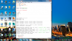
Figure 9
Whew! Now that you have entered in that code, your IDE window should resemble that of Figure 9. Press F5 to run your program. It will simulate your quad copter path and battery data like as shown in Figure 10. In the for loop where it says “rate(50)” feel free to write in your own rate. The higher the number is, the faster it will simulate. Have fun!
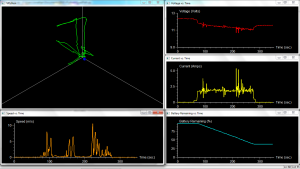
Figure 10